Demystifying the Scopes: Why Scope 3 is the True Battleground for Industrial Decarbonization
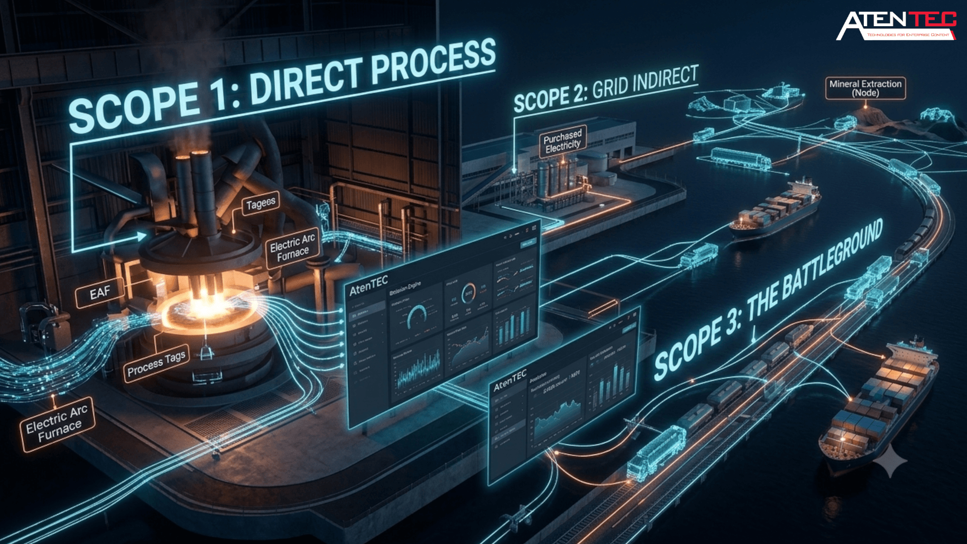
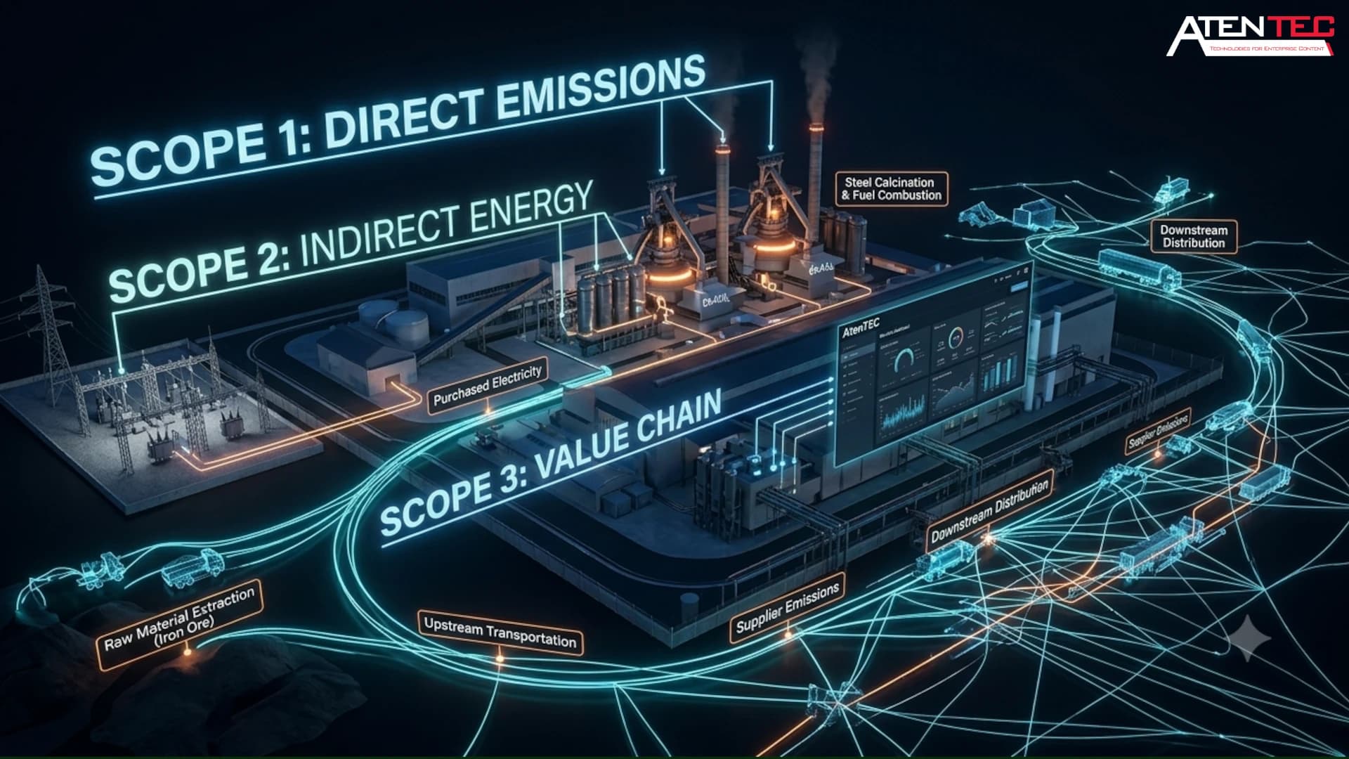
To the uninitiated, corporate carbon reporting looks like a straightforward accounting exercise. The Greenhouse Gas (GHG) Protocol neatly divides emissions into three distinct buckets: Scope 1 (direct emissions from owned sources), Scope 2 (indirect emissions from purchased energy), and Scope 3 (all other indirect emissions in the value chain). On paper, this classification system is clean, intuitive, and highly organized.
In the physical reality of heavy industrial operations, however, these boundaries are anything but clean. They represent a complex, overlapping web of thermodynamics, supply chain logistics, and volatile utility grids.
For heavy manufacturers—such as metals, chemical, and cement production facilities—treating the three scopes as isolated columns on a spreadsheet is a strategic error. Real-world decarbonization cannot occur in silos. To build a resilient, future-proof industrial enterprise, executives must understand the precise physical engineering behind each scope and recognize why Scope 3, despite being the hardest to measure, is the true battleground where global market competitiveness will be decided.
To illustrate this systemic reality, let us dissect the operational footprint of a modern, large-scale manufacturing facility specializing in structural metal production.
Scope 1: The Direct Thermodynamic Reality
Scope 1 emissions are the direct result of physical and chemical transformations occurring within the boundary of your factory walls. They are the immediate byproduct of combustion, process reactions, and fugitive escapes. In heavy industry, these emissions are not merely a consequence of turning on a machine; they are fundamentally woven into the chemistry of the manufacturing process itself.
In our industrial manufacturing example, direct emissions are heavily concentrated in the reduction and melting phases. Consider a facility utilizing a Direct Reduced Iron (DRI) shaft furnace coupled with an Electric Arc Furnace (EAF).
To reduce iron ore pellets into highly metallized sponge iron, the DRI furnace consumes massive volumes of natural gas as both a thermal fuel and a chemical reducing agent. The chemical reaction yields direct process emissions:
- Energy Intensity: The DRI process requires approximately 10 to 12 GJ of thermal energy per metric ton of product.
- Direct Emissions: This intense thermal and chemical process generates direct emissions ranging from 0.6 to 1.8 metric tons of $CO_2$ per ton of output, depending on raw material quality and furnace thermodynamic efficiency.
These emissions are locked into the physical assets of the plant. Optimizing Scope 1 is not a software configuration trick; it requires continuous, high-fidelity monitoring of thermodynamic processes. If a burner is operating at sub-optimal air-to-fuel ratios, or if a fugitive valve leaks methane, direct emissions spike instantly.
An industrial enterprise cannot manage this dynamic reality through retroactive, manual calculations. It requires direct integration with SCADA systems and edge flow meters to capture thermodynamic shifts as they happen.
Scope 2: The Grid Liability and Temporal Variance
Scope 2 emissions represent the indirect carbon liabilities you inherit when you purchase electricity, steam, or heating from third-party utility providers. While these emissions physically occur at a remote power plant, they are legally and financially attributed to your operational footprint.
For an EAF-equipped manufacturing plant, electricity is the lifeblood of the operation. The EAF uses high-voltage electric currents to melt sponge metal and recycled scrap.
- Electricity Consumption: Melting and refining one metric ton of structural metal in a modern EAF consumes roughly 500 kWh of electricity.
- The Grid Factor: The carbon footprint of this electricity is entirely dependent on the energy mix of the regional grid at the exact hour of consumption.
If the plant operates during midday in a region with high solar penetration, the local grid emission factor might be relatively low—say, 0.15 kg $CO_2$/kWh. However, if the plant runs its melting cycles during evening peak hours when the grid relies heavily on coal or natural gas-fired peaker plants, the emission factor can surge to 0.55 kg $CO_2$/kWh.
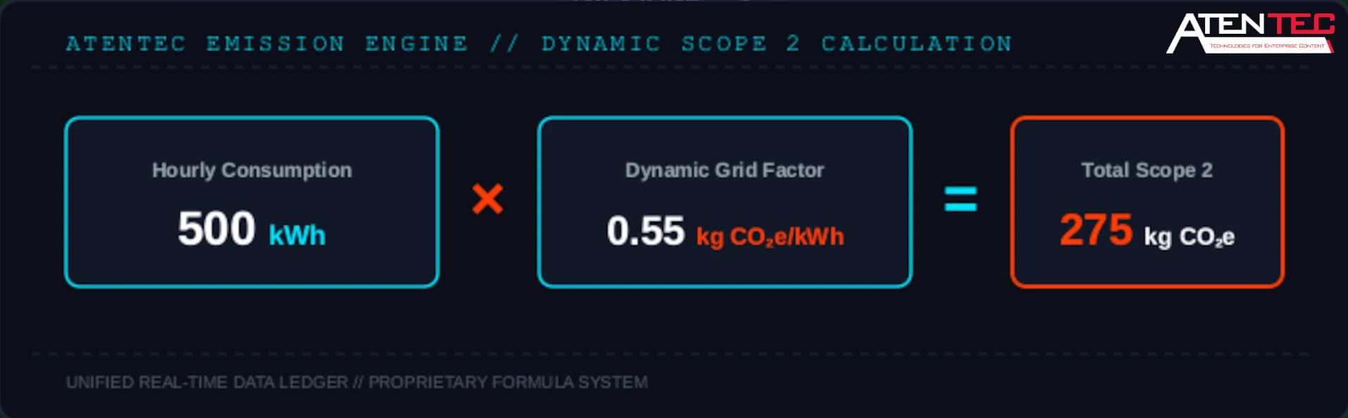
If the plant relies on a static, annualized average grid factor for its calculations, it completely misses this dynamic volatility. It pays the same carbon "price" on paper regardless of when it consumes power.
True Scope 2 optimization requires real-time grid telemetry integration. By aligning energy-intensive melting cycles with periods of low-carbon grid intensity, manufacturers can dramatically lower their real-world carbon liabilities without halting production.
Scope 3: The Untamed Wilderness of the Value Chain
Scope 3 emissions represent the entire ecosystem surrounding your business. This includes the upstream extraction and transport of your raw materials, and the downstream distribution, use, and end-of-life treatment of your products.
In heavy manufacturing, Scope 3 is almost always the largest, most complex, and most volatile portion of the carbon footprint. Yet, it is the area where companies have the least direct operational visibility.
Returning to our structural metal plant, the upstream Scope 3 boundary encompasses:
- The mining of raw ores from remote global mines.
- The processing of those ores into high-grade oxide pellets.
- The transoceanic shipping and overland rail logistics required to transport millions of tons of raw material to the facility.
When we aggregate the physical chemistry of the entire value chain, the data reveals a striking structural imbalance. While direct Scope 1 and Scope 2 emissions at a highly optimized EAF plant might total 0.85 metric tons of $CO_2e$ per ton of finished product, the upstream and downstream Scope 3 emissions can easily add another 1.6 to 2.0 metric tons of $CO_2e$ per ton.
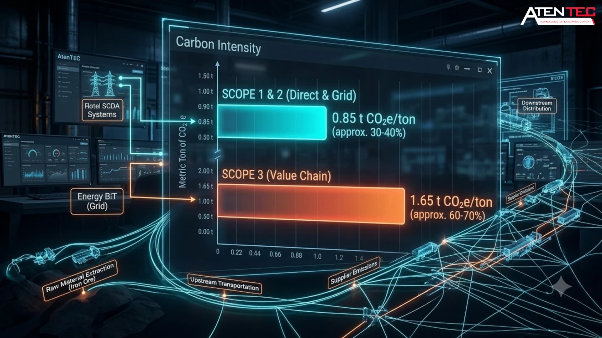
In this real-world scenario, 60% to 70% of the product's ultimate carbon liability is generated outside the factory gates.
If your procurement team makes sourcing decisions based solely on raw material purchase price, they are ignoring a massive hidden tax. Under upcoming regulatory frameworks like Europe’s Carbon Border Adjustment Mechanism (CBAM), importing raw materials with highly carbon-intensive Scope 3 supply chains will trigger severe financial penalties at the border.
If you cannot verify the exact, primary carbon data of your upstream suppliers, regulators will assign high default penalty factors to your product. In this new global economy, a lack of Scope 3 visibility is no longer just an environmental reporting failure; it is a direct threat to export revenues.
Unifying the Scopes: The AtenTEC Solution
The fundamental challenge of modern industrial decarbonization is that you cannot solve Scope 1, Scope 2, or Scope 3 in isolation. They are chemically, operationally, and financially linked.
If a manufacturing plant switches its raw material feed from direct-reduced metals (which has high Scope 1 direct emissions) to recycled scrap (which reduces Scope 1 but significantly alters melting times and electricity consumption), its Scope 2 and Scope 3 footprints instantly change. Every operational decision made on the plant floor sends shockwaves across all three boundaries.
This is why traditional, retroactively compiled spreadsheets fail. They cannot capture these multidimensional tradeoffs.
The AtenTEC Emission Engine is built to bridge this precise gap. By establishing direct, real-time data pipelines into your facility’s SCADA networks, utility meters, and ERP systems, the engine continuously monitors and visualizes the interaction between all three scopes:
- Deterministic Scope 1 & 2 Tracking: It ingests live combustion, process telemetry, and time-stamped grid factors, replacing historical averages with real-time, auditable data.
- Verified Scope 3 Integration: It provides secure data interfaces that allow your suppliers to upload primary, verified emissions profiles directly into your value chain ledger, eliminating reliance on speculative global averages.
By organizing your emissions into a unified, dynamic data model, AtenTEC transforms carbon tracking from a passive, defensive compliance obligation into an active tool for scenario simulation, strategic procurement, and global pricing optimization.
Next Step on the Journey
Now that we have mapped the dynamic relationship between Scope 1, 2, and 3 emissions, we must examine the mathematical units that define them. Join us in our next article, where we will deconstruct Emission Factors—revealing how relying on static, textbook averages creates expensive operational blind spots, and how dynamic emission profiling can save your business millions in undeserved carbon taxes.
Explore the Full Core Concepts Series
├── 1. Core Concepts 👉 Completed ✅ 👉
├── 2. Measurement Systems 👉 Previous Article
│ ├── Scope 1 / 2 / 3 👉 (You are here)
│ ├── emission factors 👉 Next Article
│ ├── lifecycle assessment (LCA) 👉 (Upcoming)
└── MRV systems 👉 (Upcoming)
Frequently Asked Questions
Why is Scope 3 considered the most critical boundary for export-oriented manufacturers?
Scope 3 emissions represent the carbon intensity of your entire supply chain, from raw material extraction to transport. Under upcoming cross-border regulations such as Europe's Carbon Border Adjustment Mechanism (CBAM), your product's total carbon liability includes these upstream emissions. If you cannot verify primary Scope 3 data, regulators apply punitive default emission factors, directly threatening your competitive pricing and export revenues.
What is the risk of using annualized grid emission factors for Scope 2 calculations?
Annualized grid factors flatten the real-world hourly volatility of the power grid. A facility running high-energy processes (like melting or thermal cracking) during peak hours inherits a much higher carbon intensity than a facility operating during off-peak, renewable-heavy hours. Relying on static, annualized averages masks this temporal variance, preventing you from optimizing electricity scheduling to lower your actual tax exposure.
How does the AtenTEC Emission Engine bridge the data gap between Scope 1 and Scope 3?
The AtenTEC Emission Engine acts as a unified data orchestrator. It ingests direct, real-time telemetry from physical shop-floor systems (SCADA, PLC, smart meters) to calculate Scope 1 and Scope 2 with absolute certainty. Simultaneously, it provides secure, API-driven data exchange layers where supply chain partners can feed verified, primary emissions data directly into your ledger—eliminating reliance on speculative global averages for Scope 3.
Can we calculate Scope 3 emissions using our existing ERP systems?
Standard ERP systems are built for financial and material flows, not high-dimensional thermodynamic and environmental data. While they can provide transaction volumes, they lack the computational architecture to trace dynamic emission profiles, verify supplier primary data, or execute real-time scenario simulation. To turn ERP data into audit-ready carbon metrics, you need a dedicated calculation layer like the AtenTEC Emission Engine.
Optimize Your Industrial Data Infrastructure
Are you ready to gain absolute visibility over your value chain emissions and secure your global export compliance? Contact the AtenTEC technical team today to evaluate your facility's operational readiness for dynamic Scope 1, 2, and 3 tracking.